

GPU utilization is often reported as one reassuring percentage. It answers whether a device was active, not whether the service delivered useful work. An inference fleet can show 85% GPU utilization while requests wait, output-token throughput stalls, and the bill climbs. That gap is where inference waste hides.
Why GPU utilization is not an inference efficiency metric
Most dashboards expose a utilization percentage sampled over time. In practice, that can mean compute activity, allocated memory, or a vendor-specific blend. None of those alone says how many requests met the latency target. A GPU can be busy reading model weights from memory while generating only a small number of tokens. It can also be busy on low-priority work while interactive traffic accumulates in a queue.
For an LLM endpoint, the useful unit is delivered output at a stated service level objective. Track tokens per second, requests per second, time to first token, and P95/P99 end-to-end latency beside GPU utilization. Then add a cost denominator: GPU-hours per million output tokens, or GPU-hours per completed request. This turns a hardware chart into an operating metric.
A simple example makes the trap clear. Imagine eight GPUs each running at 80% utilization. If a batching change raises aggregate throughput from 1,600 to 2,200 output tokens per second while P99 stays within the target, the same fleet produces 37.5% more useful work. The utilization graph might move only a few points. Conversely, a higher utilization number with flat throughput is not a win. It can signal memory stalls, queueing, or a batch policy that is too aggressive.
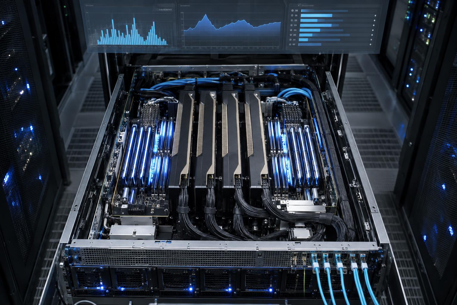
GPU utilization changes between prefill and decode
Autoregressive inference has two workload shapes. During prefill, the server processes the input prompt and builds the KV cache. That work has more parallelism and often pushes compute harder. During decode, the server emits one token per sequence per step. The model weights and KV cache move through memory repeatedly, so decode often becomes constrained by memory bandwidth rather than arithmetic throughput.
This distinction matters when reading GPU utilization. A burst of long prompts can create high prefill activity and good-looking compute charts, then leave a long decode tail where bandwidth is the limiter. A 2025 paper from IBM Research, Barcelona Supercomputing Center, and UPC found that even large-batch LLM inference can remain memory-bound because DRAM bandwidth saturates before much of the available compute does. Its authors describe a throughput knee point: after it, bigger batches add latency faster than they add throughput.
That is why VRAM occupancy is also easy to misread. High allocated memory may simply mean the KV cache is holding many live sequences. It does not prove that those sequences are progressing quickly. Low free memory can prevent useful concurrency, but a full memory graph is not an efficiency score.
Batching still matters. Larger batches amortize weight reads across more requests and can lift throughput. The cost is waiting time: an individual request may sit until the scheduler has enough compatible work. For interactive APIs, select a maximum queue delay and a P99 latency budget before increasing batch limits. For offline jobs, use a different profile that accepts longer waits in exchange for aggregate throughput.
Measure the four signals that reveal inference waste
Start with a dashboard grouped by model, hardware class, region, route, prompt-length band, and priority tier. Fleet averages erase the one shard that sets tail latency. The following signals make GPU utilization interpretable:
- Delivered throughput: output tokens per second and completed requests per GPU. Break it out by prefill and decode when the serving engine exposes those phases.
- Latency distribution: track queue time, time to first token, inter-token latency, P50, P95, and P99. A mean hides the users who see a slow response.
- Scheduler pressure: observe active sequences, waiting sequences, batch size, admission rejects, and route imbalance. A growing queue with idle devices usually points to placement or policy, not raw capacity.
- Memory and bandwidth pressure: watch KV-cache usage, cache eviction or preemption, memory bandwidth, and OOM events. These explain why high GPU utilization may not turn into more tokens.
Anyscale’s Ray Data guidance gives a concrete saturation check for batch inference: batch_size × max_concurrent_batches ≥ max_num_seqs. It uses an example with a batch size of 128 and four concurrent batches for a scheduler limit of 256 sequences. That is not a universal production setting. It is a useful way to test whether the outer pipeline feeds enough work to the serving scheduler.

Four changes worth testing before buying more GPUs
1. Separate latency classes
Do not mix a 50-token chat reply with a 20,000-token document job in one undifferentiated queue. Put interactive, batch, and premium traffic into explicit classes. Give each class a queue-delay budget and observe the resulting GPU utilization and tail latency separately. This prevents a small set of long requests from distorting the experience for everyone else.
2. Tune concurrency around the knee point
Run a controlled load sweep. Increase concurrent sequences or token budget in small steps, hold the prompt and output mix steady, and record throughput, P99, memory bandwidth, and GPU utilization. Stop when throughput flattens or the latency budget breaks. The best setting is rarely the largest batch that fits in memory.
3. Fix routing before scaling out
Compare per-replica queue time and completed tokens. One hot replica and three cool replicas means the load balancer, session affinity, prefix-cache locality, or request classification deserves attention. A capacity purchase will mask that defect while raising cost. Also inspect prompt-length skew; routing long contexts away from a latency-sensitive pool can improve the whole service.
4. Treat model choice and quantization as capacity levers
A smaller or quantized model can free memory for more live sequences, but validate quality and latency on the actual traffic mix. Measure tokens per GPU-hour before and after the change. If quantization lowers prefill time yet raises retries or output length, the apparent gain may disappear at the application layer.
A practical operating rule
Use GPU utilization as a diagnostic, not a target. A healthy deployment delivers more tokens or requests per GPU-hour while holding queue delay and tail latency inside a published budget. When that relationship weakens, look at workload mix, batching, cache pressure, and routing before assuming the fleet needs more accelerators.
For a deeper technical treatment, read the large-batch inference memory analysis, the Ray Data throughput tuning guide, and this overview of compute, memory, and bandwidth utilization. Run and scale model experiments on Wiro when the goal is measurable inference, not a flattering dashboard percentage.